Basic Reconstruction#
This tutorial shows how to use ptyrax interactively using a jupyter notebook.
We start off by some preliminary statements, which prevents resource hogging on shared computing infrastructure and sets the configuration manager (gin-config) to work interactively.
%set_env XLA_PYTHON_CLIENT_ALLOCATOR=platform

%matplotlib inline

import logging
import os
import tempfile

import gin
import jax

gin.enter_interactive_mode()
logging.basicConfig(level=logging.INFO)
tmp_dir = tempfile.mkdtemp()
# Configuring JAX to use a persistent compilation cache. This will speed up subsequent runs of the model after the first one, as compiled XLA executables will be cached on disk.
jax.config.update("jax_compilation_cache_dir", os.path.join(tmp_dir, "jax_cache"))
jax.config.update("jax_persistent_cache_min_entry_size_bytes", -1)
jax.config.update("jax_persistent_cache_min_compile_time_secs", 0)
jax.config.update("jax_persistent_cache_enable_xla_caches", "xla_gpu_per_fusion_autotune_cache_dir")
env: XLA_PYTHON_CLIENT_ALLOCATOR=platform
We start off by loading our dataset. By default, ptyrax accepts data in the cxi format, which is a specific type of hdf5 files. A cxi file may be loaded using the from_cxi(). Since there is no real standard for ptychography datasets, we will demonstrate here a more manual method of initialising a dataset. First we download the data and load it as numpy arrays.
import os
from pathlib import Path

import requests
from tqdm import tqdm

from ptyrax.utils import load_hdf5

folder = Path("data/")
filename = "lenspaper.hdf5"
data_url = "https://surfdrive.surf.nl/public.php/dav/files/sakpFtVESDmncRH"

folder.mkdir(parents=True, exist_ok=True)


def download_file_if_not_exists(url: str, output_path: Path, total_size=None, headers={}) -> None:
    if not os.path.exists(output_path):
        with requests.get(url, headers=headers, stream=True) as r:
            r.raise_for_status()

            with (
                open(output_path, "wb") as f,
                tqdm(
                    total=total_size,
                    unit="B",
                    unit_scale=True,
                    unit_divisor=1024,
                    desc="Downloading",
                ) as pbar,
            ):
                for chunk in r.iter_content(chunk_size=8192):
                    if chunk:
                        f.write(chunk)
                        pbar.update(len(chunk))

            known_size = os.path.getsize(output_path)
            logging.info(f"Downloaded {output_path} ({known_size} bytes)")
    else:
        logging.info(f"Data for {output_path} already exists, skipping download.")


dataset_path = folder / filename
download_file_if_not_exists(data_url, dataset_path, {})

data = load_hdf5(dataset_path)

diffraction_patterns = data["diffraction_patterns"]
sample_positions_orig = data["sample_positions"]
pixel_size = data["pixel_size"]
propagation_distance_orig = data["propagation_distance"]
wavelength = data["wavelength"]
/home/ssenhorst1/workspace/ptyrax/.venv/lib/python3.13/site-packages/tqdm/auto.py:21: TqdmWarning: IProgress not found. Please update jupyter and ipywidgets. See https://ipywidgets.readthedocs.io/en/stable/user_install.html
  from .autonotebook import tqdm as notebook_tqdm
INFO:2026-06-08 11:24:18,721:jax._src.xla_bridge:822: Unable to initialize backend 'tpu': INTERNAL: Failed to open libtpu.so: libtpu.so: cannot open shared object file: No such file or directory
INFO:jax._src.xla_bridge:Unable to initialize backend 'tpu': INTERNAL: Failed to open libtpu.so: libtpu.so: cannot open shared object file: No such file or directory
INFO:root:Data for data/lenspaper.hdf5 already exists, skipping download.
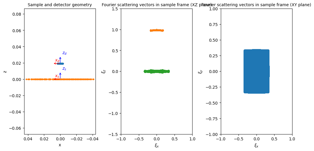
Creating the Ptychogram#
Now that we have our input data, we can generate the dataset. The dataset class is based on the CXI file format. This means that the global coordinate system is defined along the incoming beam direction. Rotations are specified as 6-dimensional vectors, equivalent to flattening the first two rows of the coordinate transformation. For more info on the rotation definition, see six_dimensional_representation_to_matrix().
Warning
To be consistent for 3-dimensional matrices, ptyrax puts the x-coordinate on the first dimension (axis 0), and the y-coordinate on the second dimension (axis 1), in contrast to most array definitions, which put the y-coordinate on the first dimension and the x-coordinate on the second. When doing manual arithmetic, it is therefore recommended to use the ptyrax.spatial module to get correct indices and rotation conventions. We can convert between the conventions once we have initialised the Ptychogram in the data using apply_orientation().
from ptyrax.spatial import SamplingGrid

detector_grid = SamplingGrid.from_tuples(diffraction_patterns.shape[1:], pixel_size)
# These are the detector x- and y-coordinates for each pixel.
xx_d, yy_d = detector_grid.meshgrid
We want to generate a Ptychogram dataset. In addition to standard keys and values, this dataset also requires exact specification of the geometry.
Note
Unless otherwise specified, all values relating to coordinates are defined in the global coordinate system. Since this system is defined along the direction of the incoming beam (following the cxi convention), coordinate directions might feel unfamiliar.
Our current dataset is a simple transmission dataset, but for good measure, we will take a more general approach to defining the coordinates, assuming a single incoming tilt rotation along the y-axis. To be general, all coordinates are defined on a per-index basis along dimension 0, so we repeat all constant values.
import jax.numpy as jnp

from ptyrax.spatial import R_y, matrix_to_six_dimensional_representation

tilt_angle = data.get("tilt_angle", 0.0)
mode = data.get("geometry", "transmission")

sample_rotation = R_y(tilt_angle)
sample_rotation = jnp.tile(sample_rotation, (diffraction_patterns.shape[0], 1, 1))
sample_orientation_6d = matrix_to_six_dimensional_representation(sample_rotation)

sample_positions = jnp.hstack((sample_positions_orig, jnp.zeros((sample_positions_orig.shape[0], 1))))
sample_positions = jnp.einsum("nij,nj->ni", sample_rotation, sample_positions)

# Detector z-axis poins in the direction of the incoming light
detector_rotation = R_y(180.0 - tilt_angle) if mode == "reflection" else R_y(0.0)
detector_rotation = jnp.tile(detector_rotation, (diffraction_patterns.shape[0], 1, 1))
detector_orientation_6d = matrix_to_six_dimensional_representation(detector_rotation)

detector_positions = detector_rotation @ jnp.array([0.0, 0.0, propagation_distance_orig])
# We assume the detector is placed perpendicular to the location where the incoming light hits the sample, which is the origin of the cxi coordinate system.
propagation_distance = jnp.tile(propagation_distance_orig, diffraction_patterns.shape[0])
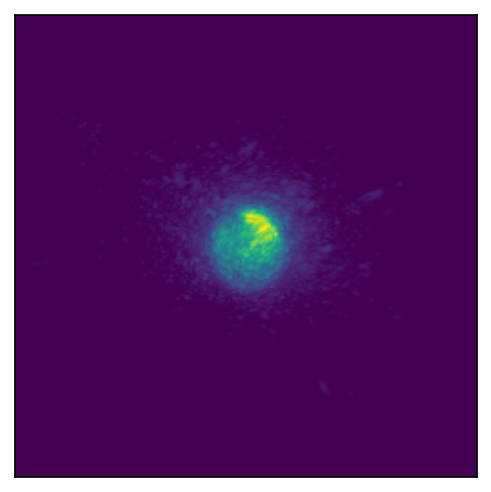
Now we have all the required geometrical parameters to generate our ptychogram! We can display the first pattern using a convencience plot function. Here we can also apply preprocessing steps. For example, to use the correct indexing convention. Check out the ptyrax.dataset module for all the transformations that may be applied to the dataset. Here we can preprocess the data. In this case, we apply 3 pre-processing steps. We flip the x- and y-axes using apply_orientation() since the coordinate definitions we take on in the code do not match the definitions that we god from the camera. We normalize the intensity using normalize_by_mean_intensity(); this is highly recommended as it makes hyperparameters and initialization values less dependent on the specific dataset. Finally we convert the data from intensity \(I\) to amplitude \(\sqrt{I}\). It is also possible to do this conversion in the forward model, but experience has taught us that this approach is more error prone when subtracting darkframes from the data.
from ptyrax.dataset import Ptychogram, apply_orientation, intensity_to_amplitude, normalize_by_mean_intensity
from ptyrax.utils import plot

ptychogram = Ptychogram(
    diffraction_patterns=diffraction_patterns,  # (N, W, H)
    pixel_size=pixel_size,  # Pixel size (2,)
    sample_positions=sample_positions,  # (N, 3)
    sample_orientations=sample_orientation_6d,  # (N, 6)
    detector_positions=detector_positions,  # (N, 3)
    propagation_distance=propagation_distance,  #
    detector_orientations=detector_orientation_6d,
    wavelength=wavelength,
)
ptychogram = apply_orientation(ptychogram, 3)
ptychogram = normalize_by_mean_intensity(ptychogram)
ptychogram = intensity_to_amplitude(ptychogram)
plot(ptychogram)
print(ptychogram)
Ptychogram loaded from Not specified with attributes:
diffraction_patterns: array of shape (202, 364, 364) and dtype float32
pixel_size: array of shape (2,) and dtype float32
sample_positions: array of shape (202, 3) and dtype float32
sample_orientations: array of shape (202, 6) and dtype float32
propagation_distance: array of shape (202,) and dtype float32
wavelength: array of shape (1,) and dtype float32
detector_positions: array of shape (202, 3) and dtype float32
detector_orientations: array of shape (202, 6) and dtype float32
loaded_from: Not specified
diffraction_pattern_scale: array of shape () and dtype float32
detector_darkframe: array of shape (364, 364) and dtype float32
mask: None
Model Initialization#
This was the hardest part, all functions afterwards are built on top of the Ptychogram abstraction. We can generate an equinox model to fit the dataset using from_image_dataset(). Equinox models are a way to combine the requirement for pure functions in JAX in a structured manner. Think of them as a way to group together state (in the form of fields of class instances), and operations which are to be performed on those fields, in the form of methods beloning to the class.
Note
Since we demand that all JAX functions are functionally pure, instances of Equinox modules are frozen: the data of a single instance cannot be modified. To make changes to Equinox modules, we have to create a new instance of the module every time we make an adjustment. This may seem to introduce a lot of overhead, but in practice this is rarely the case: all the operations we perform in the forward model are compiled to a graph; no additional copies of data are generated when this is not needed for the computation. Equinox has provided some handy methods to quickly change model fields without having to re-run the initializers. For more info, see the Equinox Docs.
from ptyrax.models.ptychography import PtychographyModel

model = PtychographyModel.from_image_dataset(ptychogram)
_ = plot(model)
INFO:root:Initializing sampling...
INFO:root:fourier_bounds=[0.33789062 0.33789062]
INFO:root:forward_fourier_bounds=[0.33789062 0.33789062]
INFO:root:forward_real_space_pixel_size=[1.3317919e-06 1.3317919e-06]
INFO:root:Pixel size anisotropy: 0.0
INFO:root:shift_bounds=array([317., 317.], dtype=float32)
INFO:root:probe_sampling.pixel_size=Array([1.3317919e-06, 1.3317919e-06], dtype=float32)
INFO:root:Initialized sampling:
Sample: shape: (998, 998)
             pixel_size: [1.3317919e-06 1.3317919e-06]
Probe: shape: (364, 364)
             pixel_size: [1.3317919e-06 1.3317919e-06]

/home/ssenhorst1/workspace/ptyrax/ptyrax/models/ptychography.py:576: UserWarning: A JAX array is being set as static! This can result in unexpected behavior and is usually a mistake to do.
  detector = detector_class(
WARNING:matplotlib.axes._base:Ignoring fixed x limits to fulfill fixed data aspect with adjustable data limits.
Tip
If you want your own equinox modules to also be plottable using the handy plot() method, you just have to implement the __plot__ function. For an example, see __plot__().
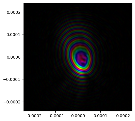
The purpose of a ptychography model is to predict the image at the detector. We can obtain its current prediction by calling it. This is where the magic happens. Check out __call__(). In accordance with the Equinox architecture, models assume their ‘batch’ dimension has already been stripped prior to calling them. Our batch dimension would usually be the current scanning position index. To facilitate this, ptyrax handles variables that are dependent on the scanning index differently; they must be resolved before the call to the model. This is taken care of by default in the training loop, but we can also do it manually. For example, if we want to obtain the current model prediction at index 0, we would do the following:
from ptyrax.parametrizations import resolve_parametrizations

model_prediction = resolve_parametrizations(model, 0)()
_ = plot(model_prediction)
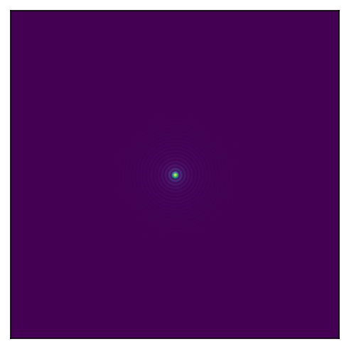
As one may guess by the diffraction pattern, the default initialization is to take the sample as a constant and the probe as a circular aperture. This can be changed in the initializer of the model. For example, to use a gaussian beam as an initializer, we use ptyrax.initializers.gaussian(). See the ptyrax.initializers module for a complete list of ptyrax.initializers.gaussian(). See the ptyrax.initializers module for a complete list of possible initializerspossible initializers.
from ptyrax.initializers import gaussian, random

model = PtychographyModel.from_image_dataset(ptychogram, probe_initializer=gaussian, interaction_initializer=random)
model_prediction = resolve_parametrizations(model, 0)()
_ = plot(model_prediction)
INFO:root:Initializing sampling...
INFO:root:fourier_bounds=[0.33789062 0.33789062]
INFO:root:forward_fourier_bounds=[0.33789062 0.33789062]
INFO:root:forward_real_space_pixel_size=[1.3317919e-06 1.3317919e-06]
INFO:root:Pixel size anisotropy: 0.0
INFO:root:shift_bounds=array([317., 317.], dtype=float32)
INFO:root:probe_sampling.pixel_size=Array([1.3317919e-06, 1.3317919e-06], dtype=float32)
INFO:root:Initialized sampling:
Sample: shape: (998, 998)
             pixel_size: [1.3317919e-06 1.3317919e-06]
Probe: shape: (364, 364)
             pixel_size: [1.3317919e-06 1.3317919e-06]
Note
Initializers are called by the model initialiser itself, as the model will determine the correct sampling to use for them. To change initialiser settings, we have to make use of some functional programming tricks. Below are two options to do this. The first is preferred, as it keeps the function named for error messages etc.
from functools import partial
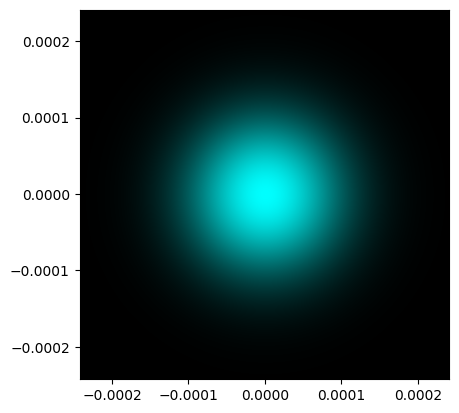
my_gaussian = partial(gaussian, radius=10.0e-5)
my_gaussian = lambda sampling, **kwargs: gaussian(sampling, radius=10.0e-5, **kwargs)
model = PtychographyModel.from_image_dataset(ptychogram, probe_initializer=my_gaussian)
plot(model.illumination)
INFO:root:Initializing sampling...
INFO:root:fourier_bounds=[0.33789062 0.33789062]
INFO:root:forward_fourier_bounds=[0.33789062 0.33789062]
INFO:root:forward_real_space_pixel_size=[1.3317919e-06 1.3317919e-06]
INFO:root:Pixel size anisotropy: 0.0
INFO:root:shift_bounds=array([317., 317.], dtype=float32)
INFO:root:probe_sampling.pixel_size=Array([1.3317919e-06, 1.3317919e-06], dtype=float32)
INFO:root:Initialized sampling:
Sample: shape: (998, 998)
             pixel_size: [1.3317919e-06 1.3317919e-06]
Probe: shape: (364, 364)
             pixel_size: [1.3317919e-06 1.3317919e-06]
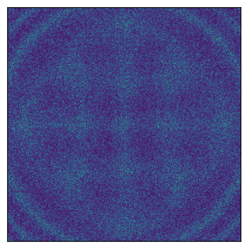
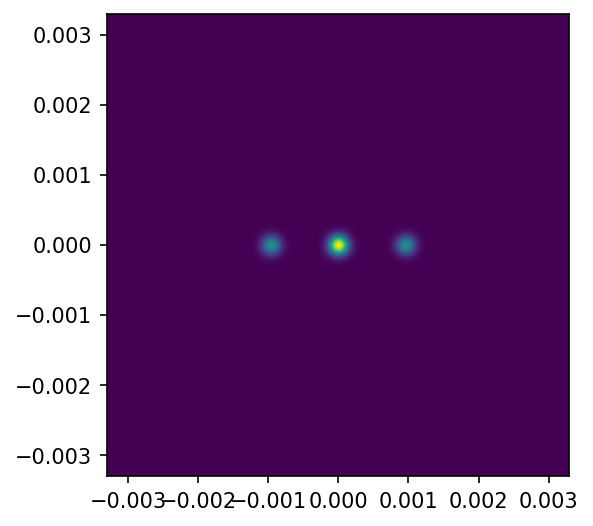
If you desire even more customization, you can create your own initializer. Initializers should have as a first argument the SamplingGrid(), and output a complex array with the shape dictated by the sampling grid. For example, we can initialize a grating-like object like this:
from jaxtyping import Array, Complex

probe_initializer = partial(gaussian, radius=2.0e-5, normalize=True)


def grating_initializer(
    sampling: SamplingGrid, period: float = 50 * wavelength, normalize=True, **kwargs
) -> Complex[Array, "m n"]:
    xx, yy = sampling.meshgrid
    grating = 0.5 * (1 + jnp.sign(jnp.cos(2 * jnp.pi * xx / period)))
    # Ptyrax assumes interaction and probes are roughly normalized. Therefore, we also normalize here.
    grating = grating / jnp.linalg.norm(grating) if normalize else grating
    return grating


def sinusoid_initializer(
    sampling: SamplingGrid, period: float = 20 * wavelength, normalize=True, **kwargs
) -> Complex[Array, "m n"]:
    xx, yy = sampling.meshgrid
    grating = 0.5 * (1 + jnp.cos(2 * jnp.pi * xx / period))
    # Ptyrax assumes interaction and probes are roughly normalized. Therefore, we also normalize here.
    grating = grating / jnp.linalg.norm(grating) if normalize else grating
    return grating


model = PtychographyModel.from_image_dataset(
    ptychogram, probe_initializer=probe_initializer, interaction_initializer=sinusoid_initializer
)
_ = plot(model.interaction)
_ = plot(resolve_parametrizations(model, 0)(), extent=model.detector.sampling.extent)
INFO:root:Initializing sampling...
INFO:root:fourier_bounds=[0.33789062 0.33789062]
INFO:root:forward_fourier_bounds=[0.33789062 0.33789062]
INFO:root:forward_real_space_pixel_size=[1.3317919e-06 1.3317919e-06]
INFO:root:Pixel size anisotropy: 0.0
INFO:root:shift_bounds=array([317., 317.], dtype=float32)
INFO:root:probe_sampling.pixel_size=Array([1.3317919e-06, 1.3317919e-06], dtype=float32)
INFO:root:Initialized sampling:
Sample: shape: (998, 998)
             pixel_size: [1.3317919e-06 1.3317919e-06]
Probe: shape: (364, 364)
             pixel_size: [1.3317919e-06 1.3317919e-06]

Reconstruction#
Now that we have a model, we of course want to optimize for it. For this, we use optax. To make optax a bit easier to use for ptychographic models, we added some helper functions to quickly generate an optimizer based off one of our models. The helper functions allow specification of different optimizers based on a pytree path, using regular expression matching. To view the pytree paths for all model parameters.
# Reset the model to a reasonable initial guess
import jax.tree


def print_all_paths(pytree, prefix: str = "") -> None:
    jax.tree.map_with_path(  # noqa: F821
        lambda path, x: logging.info(f"{prefix}{'.'.join([p.name for p in path])}"),
        pytree,
    )


model = PtychographyModel.from_image_dataset(
    ptychogram, probe_initializer=partial(gaussian, radius=(50e-6, 50e-6), normalize=True)
)

print_all_paths(model)
INFO:root:Initializing sampling...
INFO:root:fourier_bounds=[0.33789062 0.33789062]
INFO:root:forward_fourier_bounds=[0.33789062 0.33789062]
INFO:root:forward_real_space_pixel_size=[1.3317919e-06 1.3317919e-06]
INFO:root:Pixel size anisotropy: 0.0
INFO:root:shift_bounds=array([317., 317.], dtype=float32)
INFO:root:probe_sampling.pixel_size=Array([1.3317919e-06, 1.3317919e-06], dtype=float32)
INFO:root:Initialized sampling:
Sample: shape: (998, 998)
             pixel_size: [1.3317919e-06 1.3317919e-06]
Probe: shape: (364, 364)
             pixel_size: [1.3317919e-06 1.3317919e-06]

INFO:root:illumination._probe.data
INFO:root:illumination._probe.wavelength
INFO:root:illumination._probe.sampling.pixel_size
INFO:root:illumination._probe.coordinate_system.rotation._representation_6d
INFO:root:illumination._probe.coordinate_system._translation
INFO:root:illumination._probe.propagation_direction
INFO:root:interaction.coordinates.parameters.rotation._representation_6d
INFO:root:interaction.coordinates.parameters._translation._data
INFO:root:interaction.coordinates.parameters._translation._scale
INFO:root:interaction.coordinates.parameters._translation._reference_value
INFO:root:interaction.surface_normal
INFO:root:interaction.reflection_coefficient
INFO:root:interaction.sampling.pixel_size
INFO:root:interaction.sampling.origin_shift
INFO:root:interaction.forward_sampling.pixel_size
INFO:root:detector.coordinates.parameters.rotation._representation_6d
INFO:root:detector.coordinates.parameters._translation._data
INFO:root:detector.coordinates.parameters._translation._scale
INFO:root:detector.coordinates.parameters._translation._reference_value
INFO:root:detector.sampling.pixel_size
INFO:root:detector.dark_counts
Pfew! That’s a lot of parameters that we can optimize for. Let’s keep it simple for now, and just optimize for the probe (illumination._probe.data) and the object (interaction.reflection_coefficient). We must provide a list of OptimizerSpecification: each optimizer can have its own parameters it optimizes for and its own learning rate or learning rate schedule. Parameters are matched by regular expression, so for example detector.* will match all the parameters on the detector side.
from datetime import datetime

import optax

from ptyrax.training import OptimizerSpecification, initialize_optimizer_and_state

optimizer_specs = [
    OptimizerSpecification(
        name="all",
        match_patterns=[".*probe.data", ".*reflection_coefficient.*"],
        optimizer=optax.adam(1e-4),
        learn_rate_schedule=optax.constant_schedule(value=1e-4),
    )
]

optimizer_state, optimizer = initialize_optimizer_and_state(model, optimizers=optimizer_specs)
INFO:root:interaction.coordinates.parameters._translation._scale [not an array, always off]: off
Now we can optimize our model! During optimization, values are logged using Tensorboard. This allows us to keep track of previous optimization runs, and quickly compare different runs. Let’s prepare our logging…
Before we start the optimization, we should start a tensorboard server to view the progress.
Note
If you are working on a remote server, be sure that the tensorboard port is forwarded via ssh tunneling, otherwise the display will fail. In VSCode, you can forward ports using the ports view.
# One can also run a tensorboard instance externally and point it to the log directory.
# If the following cell does not run, be sure tensorboard is installed in your environment.
# You may have to run the cell twice before the output shows...
# %load_ext tensorboard
# %tensorboard --logdir logs/ --port 6006 --samples_per_plugin images=200
and start optimization!
import jax.random as jr
from tensorboardX import SummaryWriter
from ptyrax.models.ptychography import dropout, shift_probe_and_interaction
from ptyrax.reconstruct import train_model
log_dir = Path(f"logs/{datetime.now().strftime('%Y%m%d-%H%M%S')}")
log_dir.mkdir(parents=True, exist_ok=True)
writer = SummaryWriter(log_dir)
key = jr.PRNGKey(42) # We provide a key to make reconstructions reproducible. You can use any integer as the seed.
gin.bind_parameter(
"train_session.epoch_callbacks",
(
# Add removal of the shifting ambiguity by shifting to the center of mass at each epoch
shift_probe_and_interaction,
# Add dropout regularization
partial(dropout, fraction=0.2, fraction_decay=(1 / 100) ** (1 / 45), max_epoch=45),
),
)
trained_model, trained_optimizer_state = train_model(
model=model,
dataset=ptychogram,
optimizer=optimizer,
optimizer_state=optimizer_state,
num_epochs=50,
writer=writer,
key=key,
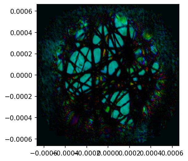
)
plot(trained_model.illumination)
plot(trained_model.interaction)
(<Figure size 900x600 with 1 Axes>,
 GridSpec(1, 1)[0:1, 0:1],
 [<matplotlib.image.AxesImage at 0x70261852da90>])
After model optimization, we can save the model in binary format as a *.eqx file, using save(). We can take a similar approach with the optimizer state, using eqx.tree_serialize_leaves.
import equinox as eqx

trained_model.save("final_model.eqx")
eqx.tree_serialise_leaves("final_optimizer_state.eqx", trained_optimizer_state)
This data can then be loaded using eqx.tree_deserialise_leaves or load().
trained_model.load("final_model.eqx")
eqx.tree_deserialise_leaves("final_optimizer_state.eqx", trained_optimizer_state)
The binary files can be a bit finnicky to load: they can only be loaded for an already instantiated model, and all the shapes have to match up. This is not always the case for ptychography, so there is also the option to save to hdf5 format, using save_model_hdf5().
from ptyrax.hdf5_checkpoint import save_model_hdf5

save_model_hdf5(trained_model, "final_model.hdf5")
This hdf5 may then be applied to an instantiated model using apply_hdf5_to_model() where the parameters have a different shape as well. The way this method deals with differing shapes can be specified per-parameter. Check out the apply_hdf5_to_model() docs for more info.
from ptyrax.hdf5_checkpoint import apply_hdf5_to_model

model = PtychographyModel.from_image_dataset(ptychogram)
model, _, _ = apply_hdf5_to_model(model, "final_model.hdf5")
INFO:root:Initializing sampling...
INFO:root:fourier_bounds=[0.33789062 0.33789062]
INFO:root:forward_fourier_bounds=[0.33789062 0.33789062]
INFO:root:forward_real_space_pixel_size=[1.3317919e-06 1.3317919e-06]
INFO:root:Pixel size anisotropy: 0.0
INFO:root:shift_bounds=array([317., 317.], dtype=float32)
INFO:root:probe_sampling.pixel_size=Array([1.3317919e-06, 1.3317919e-06], dtype=float32)
INFO:root:Initialized sampling:
Sample: shape: (998, 998)
             pixel_size: [1.3317919e-06 1.3317919e-06]
Probe: shape: (364, 364)
             pixel_size: [1.3317919e-06 1.3317919e-06]
From here, you can change optimization parameters, or start building your own models! Be sure to check out the other tutorials as well.